
 2025/09/04
In digital imaging, it is easy to assume that higher resolution automatically means better pictures. Camera manufacturers often market systems based on megapixel counts, while lens makers highlight resolving power and sharpness. Yet, in practice, image quality depends not only on the specifications of the lens or the sensor individually but also on how well they are matched.
This is where Nyquist sampling comes into play. Originally a principle from signal processing, Nyquist’s criterion sets the theoretical framework for capturing details accurately. In imaging, it ensures that the optical resolution delivered by a lens and the digital resolution of a camera’s sensor work together harmoniously.
This article unpacks Nyquist sampling in the context of imaging, explains the balance between optical and camera resolution, and provides practical guidelines for applications ranging from photography to scientific imaging.
What Is Nyquist Sampling?
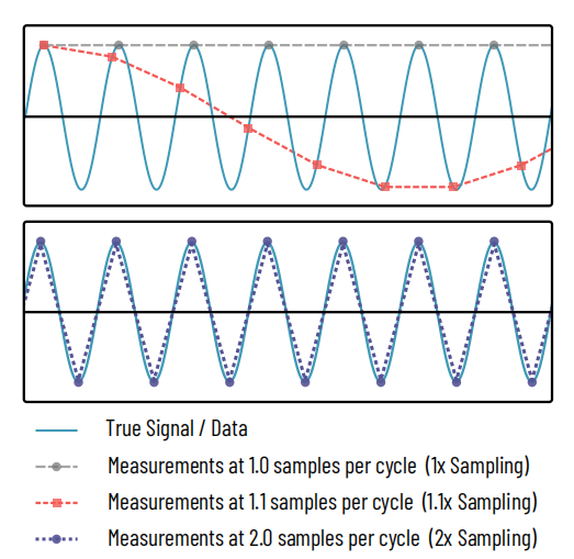
Figure 1: The Nyquist sampling theorem
Top: A sinusoidal signal (cyan) is measured, or sampled, at multiple points. The gray long-dashed line represents 1 measurement per cycle of the sinusoidal signal, capturing only signal peaks, completely hiding the true nature of the signal. The red finely dashed curve captures at 1.1 measurements per sample, revealing a sinusoid but misrepresenting its frequency. This is analogous to a Moiré pattern.
Bottom: Only when 2 samples are taken per cycle (purple dotted line) does the true nature of the signal begin to be captured.
The Nyquist sampling theorem is a principle common across signal processing in electronics, audio processing, imaging and other fields. The theorem makes clear that to reconstruct a given frequency in a signal, measurements must be made at least twice that frequency, shown in Figure 1. In the case of our optical resolution, this means that our object space pixel size must be at most half the smallest detail we are attempting to capture, or, in the case of a microscope, half the microscope’s resolution.
Figure 2: Nyquist sampling with square pixels: orientation matters
Using a camera with a grid of square pixels, the 2x sampling factor of the Nyquist theorem will only accurately capture details that are perfectly aligned to the pixel grid. If attempting to resolve structures at an angle to the pixel grid, the effective pixel size is larger, up to √2 times larger at the diagonal. The sampling rate must be therefore 2√2 times the desired spatial frequency to capture details at 45o to the pixel grid.
The reason for this is made obvious by consideration of Figure 2 (top half). Imagine the pixel size is set to the optical resolution, giving the peaks of two neighboring point sources, or any detail we are attempting to resolve, each their own pixel. Although these are then detected separately, there is no indication in the resulting measurements that they are two separate peaks – and once again our definition of "resolving" is not met. A pixel in between is needed, capturing a trough of the signal. This is achieved through at least doubling the spatial sampling rate, i.e. halving the object space pixel size.
Optical Resolution vs. Camera Resolution
To understand how Nyquist sampling works in imaging, we need to distinguish between two types of resolution:
● Optical Resolution: Determined by the lens, optical resolution refers to its ability to reproduce fine detail. Factors such as lens quality, aperture, and diffraction set this limit. The modulation transfer function (MTF) is often used to measure how well a lens transmits contrast at different spatial frequencies.
● Camera Resolution: Determined by the sensor, camera resolution depends on pixel size, pixel pitch, and overall sensor dimensions. The pixel pitch of a CMOS camera directly defines its Nyquist frequency, which determines the maximum detail the sensor can capture.
When these two are not aligned, problems arise. A lens that exceeds the resolving power of the sensor is effectively "wasted", since the sensor cannot capture all the details. Conversely, a high-resolution sensor paired with a low-quality lens results in images that do not improve despite more megapixels.
How to Balance Optical and Camera Resolution
Balancing optics and sensors means matching the Nyquist frequency of the sensor with the optical cutoff frequency of the lens.
● The Nyquist frequency of a camera sensor is calculated as 1 / (2 × pixel pitch). This defines the highest spatial frequency the sensor can sample without aliasing.
● The optical cutoff frequency depends on lens characteristics and diffraction.
For best results, the sensor’s Nyquist frequency should align with or slightly exceed the lens’s resolving ability. In practice, a good rule of thumb is to ensure the pixel pitch is about half the smallest resolvable feature size of the lens.
For example, if a lens can resolve details down to 4 micrometers, then a sensor with pixel sizes of ~2 micrometers will balance the system well.
Matching Nyquist with Camera Resolution & the Challenge of Square Pixels
The trade-off with decreasing object space pixel size is decreased light collection ability. It is therefore important to balance the need for resolution and for light collection. Additionally, larger object space pixel sizes tend to convey a larger field of view of the imaging subject. For applications that have some need for fine resolution, a ‘rule of thumb’ optimum balance is said to be struck as follows: The object space pixel size, when multiplied by some factor to account for Nyquist, should be equal to the optical resolution. This quantity is called camera resolution.
Balancing optics and sensors often comes down to ensuring that the effective sampling resolution of the camera matches the optical resolution limit of the lens. A system is said to "match Nyquist" when:
Camera resolution = Optical resolution
Where the camera resolution is given by:
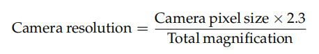
The factor to account for Nyquist that is often recommended is 2.3, not 2. The reason for this is as follows.
Camera pixels are (typically) square, and arranged on a 2-D grid. The pixel size as defined for use in the equation opposite represents the width of pixels along the axes of this grid. Should the features we are attempting to resolve lie at any angle except a perfect multiple of 90° relative to this grid, the effective pixel size will be larger, up to √2 ≈ 1.41 times the pixel size at 45°. This is shown in Figure 2 (bottom half).
The recommended factor according to the Nyquist criterion in all orientations would therefore be 2√2 ≈ 2.82. However, due to the trade-off mentioned previously between resolution and light collection, a compromise value of 2.3 is recommended as a rule of thumb.
The Role of Nyquist Sampling in Imaging
Nyquist sampling is the gatekeeper of image fidelity. When the sampling rate falls below the Nyquist limit:
● Undersampling → causes aliasing: false details, jagged edges, or moiré patterns.
● Oversampling → captures more data than the optics can deliver, leading to diminishing returns: larger files and higher processing demands without visible improvements.
Correct sampling ensures that images are both sharp and true to reality. It provides the balance between optical input and digital capture, avoiding wasted resolution on one side or misleading artifacts on the other.
Practical Applications
Nyquist sampling isn’t just theory — it has critical applications across imaging disciplines:
● Microscopy: Researchers must choose sensors that sample at least twice the smallest detail resolvable by the objective lens. Choosing the right microscopy camera is critical, as the pixel size must align with the diffraction-limited resolution of the microscope objective. Modern laboratories often prefer sCMOS cameras, which provide a balance of sensitivity, dynamic range, and fine pixel structures for high-performance biological imaging.

● Photography: Pairing high-megapixel sensors with lenses that cannot resolve equally fine details often results in negligible improvements in sharpness. Professional photographers balance lenses and cameras to avoid wasted resolution.
● Photography: Pairing high-megapixel sensors with lenses that cannot resolve equally fine details often results in negligible improvements in sharpness. Professional photographers balance lenses and cameras to avoid wasted resolution.
● Machine Vision & Scientific CamerasIn quality control and industrial inspection, missing small features due to undersampling could mean defective parts go undetected. Oversampling may be used deliberately for digital zoom or enhanced processing.
When to Match Nyquist: Oversampling and Undersampling
Nyquist sampling represents the ideal balance, but in practice, imaging systems may intentionally oversample or undersample depending on the application.
What is Undersampling
In the case of applications where sensitivity is more important than resolving the tiniest of fine details, using an object space pixel size that is larger than Nyquist demands can lead to considerable light collection advantages. This is called undersampling.
This sacrifices fine detail, but can be advantageous when:
● Sensitivity is critical: larger pixels collect more light, improving signal-to-noise ratio in low-light imaging.
● Speed matters: fewer pixels reduce readout time, enabling faster acquisition.
● Data efficiency is required: smaller file sizes are preferable in bandwidth-limited systems.
Example: In calcium or voltage imaging, signals are often averaged over regions of interest, so undersampling improves light collection without compromising the scientific outcome.
What is Oversampling
Conversely, many applications for which resolving fine details is key, or applications using post-acquisition analysis methods to recover additional information beyond the diffraction limit, require smaller imaging pixels than Nyquist demands, called oversampling.
While this does not increase true optical resolution, it can provide advantages:
● Enables digital zoom with less quality loss.
● Improves post-processing (e.g., deconvolution, denoising, super-resolution).
● Reduces visible aliasing when images are downsampled later.
Example: In microscopy, a high-resolution sCMOS camera may oversample cellular structures so that computational algorithms can extract fine details beyond the diffraction limit.
Common Misconceptions
1、More megapixels always mean sharper images.
Not true. Sharpness depends on both the lens’s resolving power and whether the sensor samples appropriately.
2、Any good lens works well with any high-resolution sensor.
A poor match between lens resolution and pixel pitch will limit performance.
3、Nyquist sampling is only relevant in signal processing, not imaging.
On the contrary, digital imaging is fundamentally a sampling process, and Nyquist is as relevant here as in audio or communications.
Conclusion
Nyquist sampling is more than a mathematical abstraction — it is the principle that ensures optical and digital resolution work together. By aligning the resolving power of lenses with the sampling capabilities of sensors, imaging systems achieve maximum clarity without artifacts or wasted capacity.
For professionals in fields as diverse as microscopy, astronomy, photography, and machine vision, understanding Nyquist sampling is key to designing or choosing imaging systems that deliver reliable results. Ultimately, image quality comes not from pushing one specification to the extreme but from achieving balance.
FAQs
What happens if Nyquist sampling isn’t satisfied in a camera?
When the sampling rate falls below the Nyquist limit, the sensor cannot represent fine details correctly. This results in aliasing, which appears as jagged edges, moiré patterns, or false textures that do not exist in the real scene.
How does pixel size affect Nyquist sampling?
Smaller pixels increase the Nyquist frequency, meaning the sensor can theoretically resolve finer details. But if the lens cannot deliver that level of resolution, the extra pixels add little value and may increase noise.
Is Nyquist sampling different for monochrome vs. color sensors?
Yes. In a monochrome sensor, every pixel samples luminance directly, so the effective Nyquist frequency matches the pixel pitch. In a color sensor with a Bayer filter, each color channel is undersampled, so the effective resolution after demosaicing is slightly lower.
Tucsen Photonics Co., Ltd. All rights reserved. When citing, please acknowledge the source: www.tucsen.com


