What Determines Image Quality in Scientific Imaging?

Image quality is often discussed as if it were a single specification—higher resolution, lower noise, or greater dynamic range. In scientific imaging, however, image quality is not defined by any one parameter. It is the result of how signal, noise, dynamic range, spatial sampling, and uniformity interact under a specific operating condition.

A camera that produces visually pleasing images may still fail in quantitative workflows if background uniformity drifts or low-signal noise limits detectability. Conversely, a system optimized for high sensitivity may sacrifice dynamic range or spatial precision.

Understanding what truly determines image quality requires a system-level perspective. This guide breaks down the physical factors that shape image quality in scientific CMOS cameras—and explains how to evaluate them based on your application.

Image Quality Is Task-Dependent

Image quality cannot be defined independently of the imaging task. The same camera may be considered excellent in one application and inadequate in another, depending on signal level, measurement objectives, and acceptable error margins. Image quality is therefore not an absolute specification—it is determined by how a system performs under specific operating conditions.

Consumer Imaging vs Scientific Imaging

In consumer photography, scenes are typically well illuminated and visually driven. Under such conditions, lens performance, spatial resolution, and color rendering dominate perceived quality. Minor fixed-pattern artefacts or small offset variations are usually masked by strong signal levels and visual contrast.

Scientific imaging operates under different constraints. In low-light environments—such as fluorescence microscopy, astronomy, or photon-limited experiments—the signal may approach only a few electrons per pixel. In these regimes, subtle noise sources, offset variation, hot pixels, glow, or structured artefacts can become visible and influence measurement reliability. The camera is no longer judged by visual appeal alone, but by its ability to preserve signal integrity.

When Do Image Quality Limitations Become Significant?

Different applications encounter different image quality challenges. High-dynamic-range inspection may prioritize linearity and uniformity. Low-light detection may prioritize read noise and dark stability. Quantitative imaging may require both precision and repeatability over time.

A practical approximation that applies across applications is this: image quality limitations become significant when systematic artefacts or non-uniformities are comparable to, or larger than, the inherent noise of the signal itself. When such effects remain well below the noise floor, their practical impact is minimal.

In short, image quality is defined by the operating regime and the precision demanded by the application—not by a single headline specification.

Signal and Noise — The Foundation of Image Quality

At its core, image quality in scientific imaging is determined by the relationship between signal and noise. No matter how advanced a sensor may be, the ability to extract meaningful information depends on how clearly the signal rises above the underlying noise floor.

Signal Level and Photoelectrons

In sCMOS cameras, image formation begins with photons generating photoelectrons in each pixel. The number of collected electrons defines the true physical signal. Digital grey values (ADU) are simply a representation of this charge after amplification and digitization. Because gain settings can change the mapping between electrons and grey levels, visual brightness alone does not define image quality—the underlying electron count does.

The signal regime matters. At high signal levels, photon shot noise dominates. At low signal levels, electronic noise sources—such as read noise and dark-related effects—become more significant.

Noise Sources in Scientific CMOS Cameras

Multiple noise components contribute to image degradation:

● Photon shot noise, which scales with the square root of the signal

● Read noise, introduced during charge-to-voltage conversion and digitization

● Dark-related variations, including DSNU (offset variation)

● Gain-related variations, such as PRNU

Each source behaves differently across signal levels. Some scale with brightness; others remain fixed. Understanding which component dominates under a given operating condition is essential for evaluating image quality realistically.

Signal-to-Noise Ratio (SNR) as a Primary Metric

Signal-to-noise ratio (SNR) provides a unifying way to assess image quality. Rather than focusing on individual specifications, SNR evaluates whether the signal of interest is distinguishable from total noise contributions.

In high-light conditions, SNR is often limited by photon statistics. In low-light regimes, SNR may be constrained by read noise or dark-related non-uniformities. As a result, improving image quality is not simply about lowering one specification—it requires identifying which noise source limits performance in the intended signal regime.

Ultimately, image quality improves when the signal increases relative to the dominant noise source. Identifying that dominant source is the first step in system-level optimization.

Dynamic Range and Contrast Reproduction

Dynamic range describes the span between the smallest detectable signal and the largest signal a sensor can record before saturation. It defines how much contrast variation an imaging system can capture in a single exposure.

Full Well Capacity and the Noise Floor

At the upper end of dynamic range lies the sensor’s full well capacity—the maximum number of electrons a pixel can store before saturating. At the lower end lies the noise floor, determined by read noise and dark-related contributions.

The ratio between full well capacity and the effective noise floor defines the usable dynamic range. A camera with low read noise but limited full well may excel in low-light detection, while a camera with high full well capacity may better capture scenes containing both bright and dim features simultaneously.

High-Light vs Low-Light Tradeoffs

Optimizing a camera for extreme sensitivity often reduces maximum charge capacity or increases gain, which can compress usable dynamic range. Conversely, optimizing for large dynamic range may compromise low-signal detectability.

As a result, image quality must be evaluated relative to the expected signal regime. A system designed for dim fluorescence imaging prioritizes low noise. A system intended for bright-field inspection may prioritize dynamic range and linearity.

Bit Depth Does Not Equal Dynamic Range

Bit depth defines how finely the analog signal is digitized, but it does not create dynamic range on its own. If the analog noise floor is high, increasing bit depth only subdivides noise more precisely—it does not extend the detectable signal range.

True dynamic range is determined by sensor physics and noise characteristics, not by digital resolution alone.

Uniformity and Fixed Pattern Artefacts

Beyond signal strength and dynamic range, image quality is also influenced by spatial uniformity. Even when noise levels are low, structured artefacts across the sensor can affect background consistency and quantitative reliability.

Offset and Gain-Related Non-Uniformity

In CMOS cameras, certain non-uniformities appear as static or repeatable patterns. These artefacts are often referred to as fixed pattern noise (FPN) because their spatial structure does not change from frame to frame.

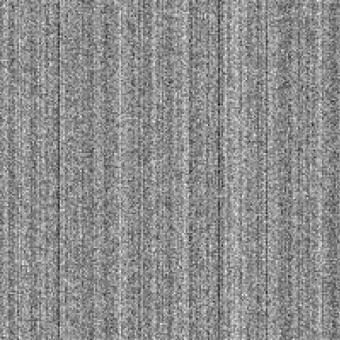
Figure 1: Fixed pattern column noise

Differences in CMOS analogue to digital converter offset value from column to column result in a visible pattern of bright and dark columns that does not change between successive frames. Seen here without incident light. This pattern can be significant compared to imaging subject contrast in low light conditions, becoming visible over images.

One common source is column-related offset variation. Many CMOS architectures use column-parallel readout, where each column is processed by a dedicated analog-to-digital converter (ADC). Small differences between ADC offsets can create visible vertical banding under low-light or bias conditions. In split-sensor designs, a horizontal division across the frame may also appear.

Less commonly, row-related patterns can occur when rows are read in parallel with slight offset mismatches. While these patterns may be subtle, the human visual system is particularly sensitive to structured repetition, making them more noticeable than purely random noise.

When Do Structured Artefacts Affect Image Quality?

Offset-related fixed patterns are most visible in low-signal regimes, where the underlying signal does not mask spatial variation. In older or lower-grade systems, such artefacts may become visible even at moderate signal levels. In modern, well-calibrated sCMOS cameras, column and row patterns are typically reduced to levels below read noise and are therefore not perceptible in standard imaging conditions.

However, structured artefacts can become more apparent in workflows involving frame averaging, background subtraction, or automated analysis. Because such patterns are systematic, they do not average away like random noise.

Why Specifications May Not Reveal Structured Patterns

Unlike DSNU, which quantifies offset variation statistically, structured patterns are not fully captured by a single RMS value. Specification sheets rarely include representative low-light bias images, making it difficult to assess structured artefacts from numbers alone.

In applications where uniformity is critical, empirical evaluation—particularly under low-signal or averaged conditions—may be necessary to confirm that spatial artefacts do not influence analysis.

Resolution Is Not the Same as Image Quality

Resolution is often mistaken as the primary indicator of image quality. While spatial resolution defines how finely details can be sampled or distinguished, it does not guarantee meaningful or accurate data.

Higher pixel counts or smaller pixel sizes increase sampling density, but they do not reduce noise, improve dynamic range, or enhance uniformity. If the signal-to-noise ratio is low, increasing resolution may simply divide noise into smaller pixels without improving detectability. In extreme low-light imaging, larger pixels with higher full well capacity and lower read noise may produce better overall image quality, even if nominal resolution is lower.

True system resolution also depends on optics, magnification, and sampling conditions—not just sensor specifications. An imaging system is limited by its weakest component.

In scientific imaging, resolution contributes to image quality, but only in balance with noise performance, dynamic range, and stability. More pixels alone do not ensure better data.

Putting It Together — How to Evaluate Image Quality

Evaluating image quality in scientific imaging requires more than reading a single specification. A systematic approach helps identify which factors truly matter for a given application.

1. Define the signal regime.

Determine whether your system operates in a photon-limited, read-noise-limited, or high-signal environment. The dominant noise source changes with signal level, and so does the relevant performance metric.

2. Identify the limiting factor.

At low signal levels, read noise and dark-related effects often dominate. At high signal levels, dynamic range, linearity, or uniformity may become more important. Improving a non-limiting specification rarely improves real image quality.

3. Evaluate spatial consistency.

Assess whether fixed pattern artefacts or non-uniformities are significant relative to the noise floor. Structured variations can affect quantitative workflows even when overall noise appears low.

4. Consider system context.

Optics, illumination stability, and calibration strategy all influence final image quality. Sensor performance cannot be evaluated in isolation from the imaging system.

Ultimately, image quality is defined not by the highest specification, but by how well the system preserves meaningful signal under real operating conditions.

Application Examples

Image quality priorities vary significantly across scientific and industrial applications. The dominant limiting factors depend on signal regime, measurement objectives, and tolerance for systematic error.

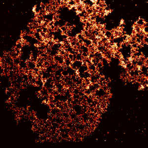
Fluorescence Microscopy

In fluorescence imaging—particularly in single-molecule fluorescence experiments—signal levels may approach only a few electrons per pixel. Image quality is therefore strongly influenced by read noise, dark stability, and background uniformity. Structured offset artefacts or hot pixels can interfere with weak signal detection and quantitative intensity analysis. In this regime, sensitivity and low-noise performance typically outweigh extreme dynamic range.

Semiconductor Inspection

Inspection systems often operate at moderate to high signal levels but require excellent uniformity and repeatability. Even subtle gain or offset variations can influence defect detection thresholds or background subtraction accuracy. Here, linearity, dynamic range, and spatial consistency are often more critical than raw sensitivity.

Conclusion

Image quality in scientific imaging is not defined by a single specification. It emerges from the balance between signal level, noise sources, dynamic range, spatial resolution, and uniformity under real operating conditions. The same camera may perform differently depending on whether the system is photon-limited, dynamic-range-limited, or constrained by spatial consistency requirements. Meaningful evaluation therefore requires understanding the dominant noise regime and the precision demanded by the application.

At Tucsen, image quality is addressed as a system-level engineering challenge—considering sensor physics, calibration strategy, and application-specific constraints. If your workflow demands quantitative reliability or extreme sensitivity, our team can help evaluate performance in the context that truly matters.