
 2025/10/20
In scientific imaging, whether in microscopy, astronomy, or semiconductor inspection, resolution is a fundamental concept that directly influences the quality and usefulness of the data captured. Simply put, resolution determines the ability of an imaging system to distinguish fine details in an object.
High resolution allows researchers to observe subtle structures, detect minor defects, or capture precise measurements, while low resolution can obscure critical information. Understanding resolution requires more than just counting pixels. Factors like optics, illumination, and sensor performance all contribute to the effective resolution of a system.
What Is Resolution in Scientific Imaging?
In consumer photography, computer and smartphone screens, and video streaming, the term 'resolution' typically refers to pixel count. Terms like '720p', '1080p' and '4K' define resolution by the number of horizontal rows of pixels, while describing a smartphone camera as ‘20MP’ implies it has 20 million pixels.
In scientific imaging though, the term 'resolution' means something different, and specific. Namely, the ability to optically 'resolve' fine spatial details in the image from each other. This depends on both the optical setup, and the pixel size of the camera used. Under this definition, it is field of view – not resolution – that is defined by the pixel count of our camera sensor.
At some level, all light information captured by a camera is 'blurred' by diffraction and aberrations – whether this is due to imperfect optics, or to the physical limitations due to the wavelength of light, there is a limit on our capturing of details that means the perfect ‘ground truth’ is forever beyond our reach. The optical resolution is the smallest level of detail that is actually preserved.
Further, our camera’s pixels are not infinitely small – above some key lengthscale, images will become 'pixelated'. This additional factor, the ‘camera resolution’, interacts with the optical resolution to define the overall resolution of our system.
Defining Optical Resolution – Diffraction-Limited Resolution
If we had a perfect lens, with no defects, aberrations or design flaws, would we be able to resolve any detail no matter how small? In reality, no matter the quality of our lens, the physics of light waves will provide an upper limit to the resolving power of lenses and microscope objectives.
The diffraction of light causes blurring on a length scale that depends upon the wavelength of light used, and the aperture size of the lenses used for illumination and imaging. If an infinitely small but bright 'point source' of light was imaged by a lens, the resulting image would be blurred into a characteristic shape called the Airy disk shown in Figure 1.
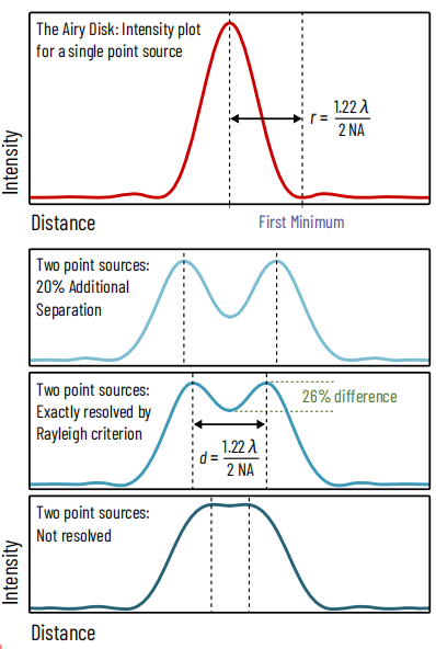
Figure 1: Defining resolution: the Rayleigh criterion
A point source of light is spread by optical components to form an image known as the 'airy disk'. In microscopy, the size of this disk is determined by the wavelength of light and the numerical aperture of the objective (in reflected light mode, e.g., fluorescence).
The Rayleigh criterion for whether two point sources are resolved is met if the distance between them is at least the distance to the first minimum of the airy disk, and the contrast ratio between the peaks and the central trough is at least 26%.
The Rayleigh Criterion
The definition of diffraction-limited resolution then is ‘how close can two point-like sources of light get to each other before they can no longer be distinguished (resolved) as two separate points?’ This is shown in Figure 1.
There are a number of mathematical conventions of where exactly to draw this line, but the one most commonly used is the Rayleigh Criterion, whereby the peak of one point coincides with the first minimum of the diffraction pattern of the other point. This corresponds to a contrast ratio of 26% between the intensity of the peaks and the trough between them.
In spatial terms, the minimum resolvable length-scale can be defined as a minimum distance between points, or in angular terms as a minimum angle relative to the optical axis of a lens.
The Point Spread Function (PSF)
The actual shape of a diffraction pattern for a point light source once imaged by an optical setup is called the point spread function (PSF). In advanced microscopy, this is often measured in three dimensions. The shape of the PSF can be affected by every optical element in the lightpath, and minimizing its size to maximize resolving power is a common aim for optical engineers.
Some analysis techniques such as deconvolution usually require as an input the 3-dimensional shape of the PSF. Additionally, the shape of the PSF can be deliberately changed to encode additional information, such as the vertical (z-axis) position of the point, in a field known as PSF engineering.
Defining Optical Resolution – Limitations of Lens Quality: MTF and CTF
In practice for many optical systems, especially for lens-based imaging, the diffraction-limited resolution introduced above is a ‘best case’ scenario only approached by the highest quality lenses. Other factors, including a lengthy list of common optical aberrations, and how closely the lens manufacturers were able to match their intended precise mathematical lens shape, reduce this resolving power. Resolution then is typically defined experimentally based on measured contrast at different length scales, or by simulation and theoretical calculation taking each lens element into account.
The most common mathematical representation of resolution in this case is the Optical Transfer Function (OTF), consisting of the Modulation Transfer Function (MTF) and the Phase Transfer Function (PTF). The MTF represents how much contrast can be delivered by the lens or optical system at different length scales or spatial frequencies. The PTF won’t be examined here; imaging phase information requires specialist optical setups and can be neglected for conventional imaging. MTF can be calculated for theoretical lenses and optical setups. However, it can be hard to measure in practice.
Instead, a simpler approach can be taken for real-world testing of optical components, measuring the so-called Contrast Transfer Function (CTF).
CTF & MTF Graphs
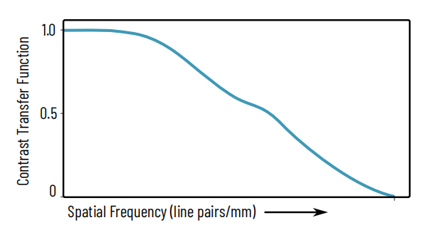
Figure 2: Example of a CTF curve
Contrast Transfer Function (CTF) is a numerical measure of the amount of contrast that passes through an optical system. X axis: spatial frequency in line pairs/mm, increasing from left to right. Real CTF and MTF measurements typically include multiple different curves corresponding to different measurement conditions, such as radial vs. parallel target lines, horizontal/vertical lines, different lens settings etc.
The CTF of a lens is a complicated function influenced by every optical element in the optical path, and can be measured for each lens, the camera sensor, or for the complete optical system. The typical form of the plot is shown in Figure 2.
The X axis is typically represented in ‘line pairs per mm’, referring to how successfully the tested component can reproduce a pair of lines, one bright and one dark, at that given spatial frequency. The inverse of this number would yield the thickness of the line pair. On the Y axis is the CTF, which is a ratio of the contrast between the lines going into the lens versus coming out of it, as in Equation 1, with contrast defined as in Equation 2.
Factors affecting MTF/CTF
For example, consider a sequence of line pairs with bright lines bordered by dark lines that were only 20% as bright. The contrast in this case would be 66% according to Equation 6. If upon passage through a lens, the bright lines were spread out by diffraction and aberrations such that now, dark lines were 50% of the intensity of the bright lines, the contrast would now be 33%, and the CTF would be 33%/66% = 50%. In most cases, the higher the spatial frequency in lp/mm, the lower the CTF – though the curve is not always monotonic (smoothly decreasing).
The MTF of a typical camera lens is dependent upon multiple factors, hence typically multiple graphs are plotted to characterize one lens. Factors include aperture size (e.g. f/4, f/8 etc.), distance from the center of the lens, and whether the line pairs measured are parallel with the grid of pixels of the camera sensor, as explored for diffraction-limited resolution.
Ultimately, the answer to the question “does this lens / sensor combination deliver enough resolution for my application” may require experimental testing and benchmarking.
Spatial Frequency: Measuring Detail
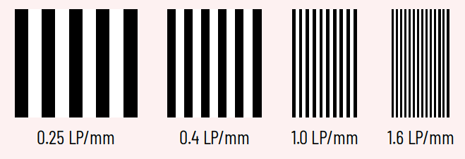
Figure 3: Example of increasing spatial frequency in line pairs / mm
Spatial frequency is a concept commonly used in discussions of resolution. It simply refers to ‘how many features exist per unit distance’, e.g., a repeating pattern of closely spaced lines. It is commonly measured in units of inverse distance, for example m-1, though inverse millimeters mm-1 is identical in practice to line pairs per mm (lp/mm). Spatial frequency is directly analogous to the ‘temporal’ frequency of light or sound waves, except measuring per unit of space, rather than time.
Resolution, Contrast, and SNR (Signal-to-Noise Ratio)
It’s important to remember that resolution calculations and measurements are a ‘best-case’ scenario. The definition of resolution above relies upon image contrast. Achieving the contrast required to resolve fine details relies on not only optical and camera resolution but on signal-to-noise ratio (SNR), background light, image quality and other factors.
It is also worth noting that factors that improve optical resolution can often also improve other important factors – for example, increasing microscope objective or lens aperture size also results in more light collection, typically improving signal-to-noise ratio. Indeed, for fluorescence imaging with a microscope objective, the brightness of the light collected depends upon numerical aperture to the fourth power, meaning a small increase in NA can lead to a significant improvement in image brightness.
Key Factors Affecting Resolution in Scientific Imaging
Beyond the theoretical limits, practical resolution is shaped by several interdependent factors:
1. Lens quality and aberrations
● Aberration correction (apochromatic lenses, adaptive optics) is essential for high-resolution imaging.
● Poor lens quality reduces MTF and broadens the PSF.
2. Numerical Aperture (NA)
● Higher NA lenses capture more diffracted light and improve resolution.
● NA is limited by physical design and the refractive index of the imaging medium.
3. Wavelength of illumination
● Shorter wavelengths (e.g., blue light) yield higher resolution.
● Techniques like super-resolution microscopy exploit this principle by manipulating effective wavelength limits.
4. Sensor characteristics
● Pixel size: Smaller pixels can sample finer details, but only if the optics deliver sufficient resolution (Nyquist sampling criterion).
● Quantum efficiency: Higher QE improves SNR, revealing finer details.
● Read noise and dark current: Low-noise sensors preserve contrast at high spatial frequencies.
5. Illumination and sample conditions
● Uneven or weak illumination reduces contrast.
● Sample preparation, staining, or labeling can directly affect the ability to resolve structures.
Conclusion
Resolution is a cornerstone of scientific imaging. It defines the ability of a system to distinguish fine details, impacting everything from microscopy to semiconductor inspection. While megapixels often dominate public perception, true resolution is determined by a combination of optics, diffraction, sensor characteristics, and image quality factors like contrast and SNR.
By understanding concepts such as the Point Spread Function, MTF, spatial frequency, and the physical limits imposed by diffraction, researchers can make informed choices about imaging systems, optimize experimental setups, and interpret results accurately. Ultimately, mastering resolution is essential for achieving high-quality, meaningful scientific images.
Tucsen Photonics Co., Ltd. All rights reserved. When citing, please acknowledge the source: www.tucsen.com


